from logistic_regression import LogisticRegression
from sklearn.datasets import make_blobs
from matplotlib import pyplot as plt
import numpy as np
np.seterr(all='ignore')

np.random.seed(1234)

# make the data
p_features = 3
X, y = make_blobs(n_samples = 200, n_features = p_features - 1, centers = [(-1, -1), (1, 1)])https://github.com/ZaynMak/zaynmak.github.io/tree/main/posts/Gradient-Descent
Introduction
In this blog post I will be demonstrating my implementation of the Gradient Descent Algorithm and show it in action for the logistic regression problem. I will also be comparing it to the Stochastic Gradient Descent Algorithm and show how it can be used to improve the performance of the Gradient Descent Algorithm. I will also be showing how the momentum feature can be used to improve the performance of the Stochastic Gradient Descent Algorithm. Then, I will perform some experiments on synthetic data to show how the learning rate, batch size and momentum affect the performance of the Stochastic Gradient Descent Algorithm.
LR = LogisticRegression()
LR.fit_stochastic(X, y, 0.01, 10, 1000)

# inspect the fitted value of w
LR.w

fig = plt.scatter(X[:,0], X[:,1], c = y)
xlab = plt.xlabel("Feature 1")
ylab = plt.ylabel("Feature 2")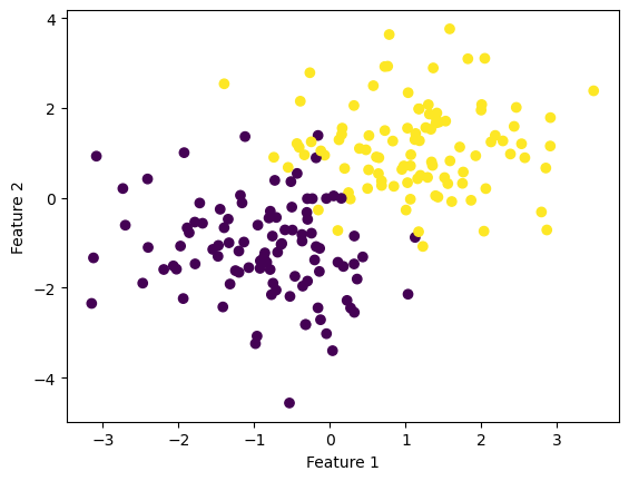
X_ = np.append(X, np.ones((X.shape[0], 1)), 1)
# calculate the loss
loss = LR.empirical_risk(X_, y)

# plot the decision boundary
fig = plt.scatter(X[:,0], X[:,1], c = y)
xlab = plt.xlabel("Feature 1")
ylab = plt.ylabel("Feature 2")

f1 = np.linspace(-3, 3, 101)

# we plot the data with the decision boundary
p = plt.plot(f1, (LR.w[2] - f1*LR.w[0])/LR.w[1], color = "black")
title = plt.gca().set_title(f"Loss = {loss}")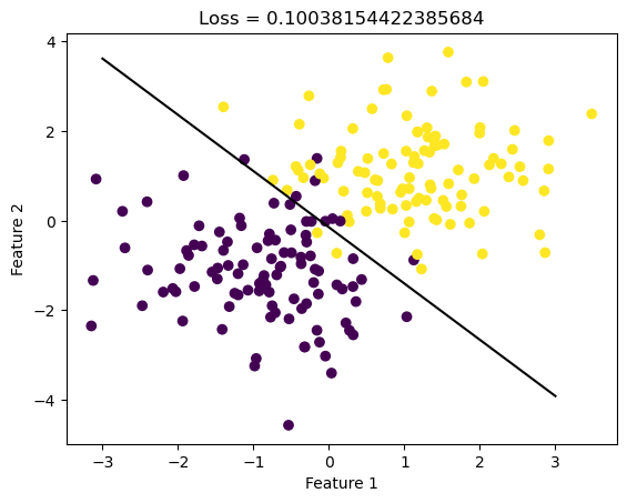
# we find the loss history for the stochastic gradient descent with momentum
LR = LogisticRegression()
LR.fit_stochastic(X, y,
                  max_epochs = 100,
                  momentum = True,
                  alpha = .05,
                  batch_size = 10)

num_steps = len(LR.loss_history)
plt.plot(np.arange(num_steps) + 1, LR.loss_history, label = "stochastic gradient (momentum)")

# we find the loss history for the stochastic gradient descent without momentum
LR = LogisticRegression()
LR.fit_stochastic(X, y,
                  max_epochs = 100,
                  batch_size = 10,
                  alpha = .5)

num_steps = len(LR.loss_history)
plt.plot(np.arange(num_steps) + 1, LR.loss_history, label = "stochastic gradient")

# we find the loss history for the gradient descent
LR = LogisticRegression()
LR.fit(X, y,
       alpha = .05,
       max_epochs = 100)

num_steps = len(LR.loss_history)
plt.plot(np.arange(num_steps) + 1, LR.loss_history, label = "gradient")

# we set it in the log space
plt.loglog()

# we set the labels
legend = plt.legend()

title = plt.gca().set_title(f"Loss History for the Different Methods")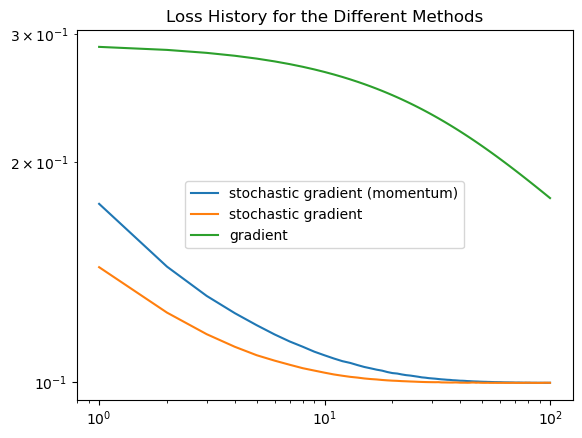
Experiment 1
I will run a stochastic gradient descent with a large alpha.
LR = LogisticRegression()
LR.fit_stochastic(X, y, 5, 10, 1000)
fig = plt.plot(LR.score_history)
xlab = plt.xlabel("Iteration")
ylab = plt.ylabel("Accuracy")
title = plt.title("Accuracy over time")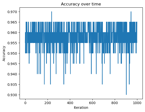
As we can see, the accuracy does not converge to 1, but rather oscillates around 0.96. This is because the learning rate is too large and the algorithm overshoots the minimum.
Experiment 2
I will now change the batch size to compare our loss history.
LR = LogisticRegression()
LR.fit_stochastic(X, y,
                  max_epochs = 100,
                  batch_size = 2,
                  alpha = .1)

num_steps = len(LR.loss_history)
plt.plot(np.arange(num_steps) + 1, LR.loss_history, label = "Batch size 2")

LR = LogisticRegression()
LR.fit_stochastic(X, y,
                  max_epochs = 100,
                  batch_size = 3,
                  alpha = .1)

num_steps = len(LR.loss_history)
plt.plot(np.arange(num_steps) + 1, LR.loss_history, label = "Batch size 3")

LR = LogisticRegression()
LR.fit_stochastic(X, y,
                  max_epochs = 100,
                  batch_size = 7,
                  alpha = .1)

num_steps = len(LR.loss_history)
plt.plot(np.arange(num_steps) + 1, LR.loss_history, label = "Batch size 7")

LR = LogisticRegression()
LR.fit_stochastic(X, y,
                  max_epochs = 100,
                  batch_size = 15,
                  alpha = .1)

num_steps = len(LR.loss_history)
plt.plot(np.arange(num_steps) + 1, LR.loss_history, label = "Batch size 15")

LR = LogisticRegression()
LR.fit_stochastic(X, y,
                  max_epochs = 100,
                  batch_size = 30,
                  alpha = .1)

num_steps = len(LR.loss_history)
plt.plot(np.arange(num_steps) + 1, LR.loss_history, label = "Batch size 30")

plt.loglog()

legend = plt.legend() 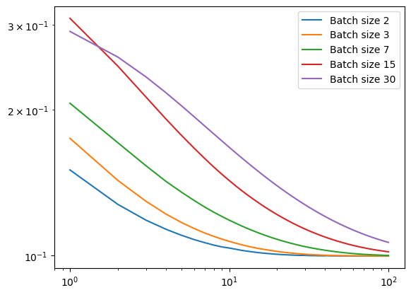
We see that the fastest decrease in loss is for batch size 2, but it also starts at the lowest starting loss value.
Experiment 3
I will now compare stochastic gradient descent with and without momentum’s loss history.
# we create data with 10 features
p_features = 10
X, y = make_blobs(n_samples = 200, n_features = p_features - 1, centers = [(-1, -1), (1, 1)])

# we find the loss history for the stochastic gradient descent with momentum
LR = LogisticRegression()
LR.fit_stochastic(X, y,
                    max_epochs = 100,
                    momentum = True,
                    alpha = .05,
                    batch_size = 10)

num_steps = len(LR.loss_history)
plt.plot(np.arange(num_steps) + 1, LR.loss_history, label = "stochastic gradient (momentum)")

# we find the loss history for the stochastic gradient descent without momentum
LR = LogisticRegression()
LR.fit_stochastic(X, y,
                    max_epochs = 100,
                    momentum = False,
                    alpha = .05,
                    batch_size = 10)

num_steps = len(LR.loss_history)
plt.plot(np.arange(num_steps) + 1, LR.loss_history, label = "stochastic gradient")

# we plot it in the log space
plt.loglog()

# we set the labels
legend = plt.legend()

# set the title
title = plt.gca().set_title(f"Loss History for the Stochastic Gradient Descent with and without Momentum")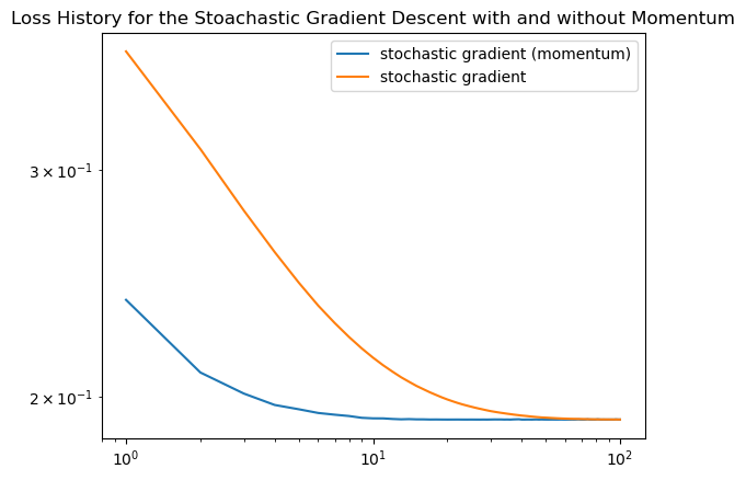
We see that stochastic gradient descent with momentum has a much faster decrease in loss than stochastic gradient descent without momentum.
Conclusion
I have compared the three algorithms and shown how they can be used to solve the logistic regression problem. I have also shown how the learning rate, batch size and momentum affect the performance of the stochastic gradient descent algorithm.